library(statnet) # also loads the ERGM package
library(igraph)
library(ggraph)
library(intergraph)
library(patchwork)
library(networkdata)Social Network Analysis
Worksheet 10: ERGMs I
Introduction
We’re going to follow the ERGM modelling outline:
- specify and estimate model parameters that should govern evolution of network
- simulate other random networks based on specified models
- compare the goodness of fit of observed to model networks.
The following resource is useful for looking up different model terms: ERGM terms.
Note that we now are performing stochastic simulation – in some of the cases, your output will differ slightly from mine and between different runs (you can however use set.seed() to get exactly the same results).
Packages needed
Object types
We will be primarily be working with matrix, network and graph objects. Note that ergm primarily requires network and adjacency matrices, but since we will be using ggraph to visualize networks we also need graph objects. We try to keep it clear here by using suffix g, net and mat to clarify object assignment.
Florentine marriage network
We start by loading the Florentine marriage network (available in the statnet package) and create the adjacency matrix from the loaded network object. This is done with the below code. Note that we have some available node attributes: priorates, totalties, vertex.names and wealth. We’ll be using these attributes later for modeling ERGMs.
data(florentine) # loads flomarriage and flobusiness data
flom_net <- flomarriage # look at the flomarriage network data
flom_mat <- as.matrix(flomarriage)To visualize the network we create a graph object (note that using geom_node_text includes the vertex/family names but you can exclude this if you prefer):
flom_g <- asIgraph(flom_net)
flom_p <- ggraph(flom_g, layout = "stress") +
geom_edge_link0(edge_colour = "#666060",
edge_width = 0.8, edge_alpha = 1) +
geom_node_point(fill = "#808080", colour = "#808080",
size = 7, shape = 21, stroke = 0.9) +
theme_graph() +
theme(legend.position = "none") +
geom_node_text(aes(label = vertex.names), colour = "#000000",
size = 5, family = "sans") +
ggtitle("Florentine marriage network")
flom_p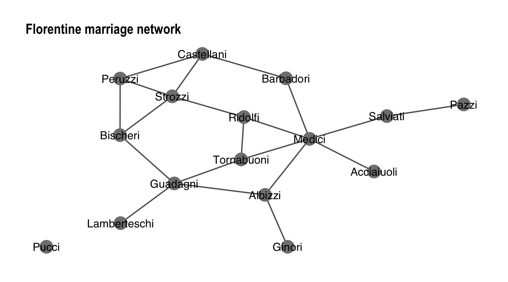
Model 1: Dyadic independence/Bernoulli graph
Estimation
We begin by specifying a Bernoulli model using the ergm function. This is done by only including number of edges as a term in the model (recall from lecture that this implies dyadic independence). Run the model and print out summary of model fit using below code:
flom_mod1 <- ergm(flom_net ~ edges) # fit the model
summary(flom_mod1) # get a summary of modelCall:
ergm(formula = flom_net ~ edges)
Maximum Likelihood Results:
Estimate Std. Error MCMC % z value Pr(>|z|)
edges -1.6094 0.2449 0 -6.571 <1e-04 ***
---
Signif. codes: 0 '***' 0.001 '**' 0.01 '*' 0.05 '.' 0.1 ' ' 1
Null Deviance: 166.4 on 120 degrees of freedom
Residual Deviance: 108.1 on 119 degrees of freedom
AIC: 110.1 BIC: 112.9 (Smaller is better. MC Std. Err. = 0)You can also just print the estimated coefficient using only flom_mod1.
Q1. How can you interpret the parameter estimate?
The log-odds of any tie occurring is: \[ -1.609 \times \textrm{change in the number of ties} = -1.609 \times 1 \] for all ties, since the addition of any tie to the network changes the number of ties by 1. Corresponding probability is: \[\frac{\exp{(-1.609)}}{1+\exp{(-1.609)}}=0.1667\] which is what you would expect, since there are 20/120 ties.
Model 2: Transitivity effect added
Estimation
Next, we add a term the number of completed triangles/triads (which would indicate transitivity).
set.seed(1) #include if you want the same results shown here
flom_mod2 <- ergm(flom_net ~ edges + triangle)
summary(flom_mod2) Call:
ergm(formula = flom_net ~ edges + triangle)
Monte Carlo Maximum Likelihood Results:
Estimate Std. Error MCMC % z value Pr(>|z|)
edges -1.6913 0.3219 0 -5.254 <1e-04 ***
triangle 0.1808 0.5567 0 0.325 0.745
---
Signif. codes: 0 '***' 0.001 '**' 0.01 '*' 0.05 '.' 0.1 ' ' 1
Null Deviance: 166.4 on 120 degrees of freedom
Residual Deviance: 108.1 on 118 degrees of freedom
AIC: 112.1 BIC: 117.6 (Smaller is better. MC Std. Err. = 0.01061)Q2 How can you interpret the parameter estimates?
Q3 What do the parameter estimates tell us about the configurations specified in the model?
Conditional log-odds of two actors forming a tie is:
- \(-1.6913\times\) change in the number of ties + \(0.1808 \times\) change in number of triangles
- if the tie will not add any triangles to the network, its log-odds is: -1.6913
- if it will add one triangle to the network, its log-odds is: -1.6913 + 0.1808
- if it will add two triangles to the network, its log-odds is: -1.6913 + 0.1808 \(\times\) 2
MCMC diagnostics
You can use mcmc.diagnostics(flom_mod2) to observe the behavior of the MCMC estimation algorithm and check for degeneracy. What you want to see in the MCMC diagnostics: the MCMC sample statistics varying randomly around the observed values at each step in the trace plots (which means the chain is mixing well) and the difference between the observed and simulated values of the sample statistics should have a roughly bell-shaped distribution, centered at 0 (which means no difference):
mcmc.diagnostics(flom_mod2, center = TRUE)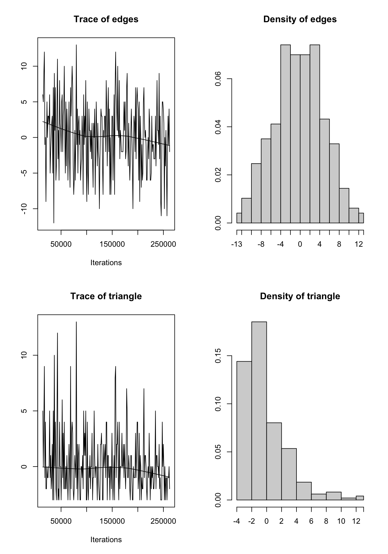
Sample statistics summary:
Iterations = 14336:262144
Thinning interval = 1024
Number of chains = 1
Sample size per chain = 243
1. Empirical mean and standard deviation for each variable,
plus standard error of the mean:
Mean SD Naive SE Time-series SE
edges 0.2058 4.957 0.3180 0.3180
triangle 0.2222 2.866 0.1839 0.1839
2. Quantiles for each variable:
2.5% 25% 50% 75% 97.5%
edges -9 -3 0 4 9.95
triangle -3 -2 0 1 7.95
Are sample statistics significantly different from observed?
edges triangle (Omni)
diff. 0.2057613 0.2222222 NA
test stat. 0.6471018 1.2086209 1.6694087
P-val. 0.5175661 0.2268085 0.4367585
Sample statistics cross-correlations:
edges triangle
edges 1.0000000 0.7771561
triangle 0.7771561 1.0000000
Sample statistics auto-correlation:
Chain 1
edges triangle
Lag 0 1.000000000 1.00000000
Lag 1024 0.056425983 -0.04043396
Lag 2048 0.006273791 0.01940035
Lag 3072 -0.051649675 -0.02455474
Lag 4096 -0.034487041 0.02913158
Lag 5120 -0.023329356 0.01178056
Sample statistics burn-in diagnostic (Geweke):
Chain 1
Fraction in 1st window = 0.1
Fraction in 2nd window = 0.5
edges triangle
1.458524 1.483872
Individual P-values (lower = worse):
edges triangle
0.1446962 0.1378428
Joint P-value (lower = worse): 0.1011719
Note: MCMC diagnostics shown here are from the last round of
simulation, prior to computation of final parameter estimates.
Because the final estimates are refinements of those used for this
simulation run, these diagnostics may understate model performance.
To directly assess the performance of the final model on in-model
statistics, please use the GOF command: gof(ergmFitObject,
GOF=~model).Q4 How would you interpret these results?
Simulation
When we have estimated the coefficients of an ERGM, we have defined a probability distribution across all networks of the same size. If the model is a good fit to the observed data, networks drawn from this distribution resemble the observed data. To draw networks from this distribution we use the simulate() function. We draw ten networks from the specified model and use the below command to get a summary of what the network statistics edges and triangles are for each of the ten sampled networks.
flom_mod2.sim <- simulate(flom_mod2, nsim = 10)
summary(flom_mod2.sim)List of 10 Networks
Model: flom_net ~ edges + triangle
Reference: ~Bernoulli
Constraints: ~. ~. - observed
Stored network statistics:
edges triangle
[1,] 16 3
[2,] 26 7
[3,] 18 1
[4,] 17 1
[5,] 22 1
[6,] 18 1
[7,] 11 1
[8,] 22 4
[9,] 20 3
[10,] 26 6
attr(,"monitored")
[1] FALSE FALSEList of 10 Networks
Model: flom_net ~ edges + triangle
Reference: ~Bernoulli
Constraints: ~. ~. - observed This should give you a list over the ten networks and columns representing how many edges and triangles are apparent in each simulated case. Since you have listed all the simulated networks, you can simply call each one of them individually. For example, in the below, we call simulated networks 1 and 2:
flom_mod2.sim[[1]]
flom_mod2.sim[[2]]You can also choose one of the networks to visualize, below is an example for the tenth, i.e. last on the list of, simulated network:
flom.sim_g <-asIgraph(flom_mod2.sim[[10]])
flom.sim_p <- ggraph(flom.sim_g, layout = "stress") +
geom_edge_link0(edge_colour = "#666060",
edge_width = 0.8, edge_alpha = 1) +
geom_node_point(fill = "#808080", colour = "#808080",
size = 7, shape = 21, stroke = 0.9) +
theme_graph() +
theme(legend.position = "none") +
ggtitle("Simulated network")
flom.sim_p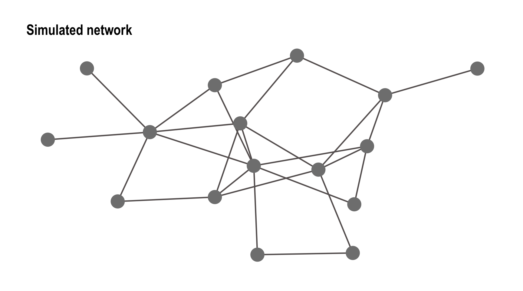
These simulations are crucial for examining the goodness of fit which we will do next.
3. Goodness of Fit
The MCMC algorithm draws a dyad at random at each step, and evaluates the probability of a tie from the perspective of these two nodes. That probability is governed by the ergm-terms specified in the model, and the current estimates of the coefficients on these terms. Once the estimates converge, simulations from the model will produce networks that are centered on the observed model statistics i.e. those we control for (otherwise it is a sign that something has gone wrong in the estimation process). The networks will also have other emergent global properties that are not represented by explicit terms in the model. Thus, goodness of fit can be done in two ways, where the first is to be preferred:
evaluate the fit to the specified terms in the model (done by default)
evaluate the fit of terms not specified in the model to emergent global network properties
If the first does not indicate something off in the estimation process, you can use the second where three terms that can be used to evaluate the fit to emergent global network properties:
the node level (degree)
the edge level (esp: edgewise share partners)
the dyad level (geodesic distances)
We check now whether the specified model above fits the observed data and how well it reproduces it. We do this by choosing a network statistic (that is not specified in the model), and comparing the value of this statistic to the distribution of values we get in simulated networks from our model. We use the gof() function.
flom_mod2.gof <- gof(flom_mod2) # this will produce 4 plots
par(mfrow=c(2,2)) # figure orientation with 2 rows and 2 columns
plot(flom_mod2.gof) # gof plots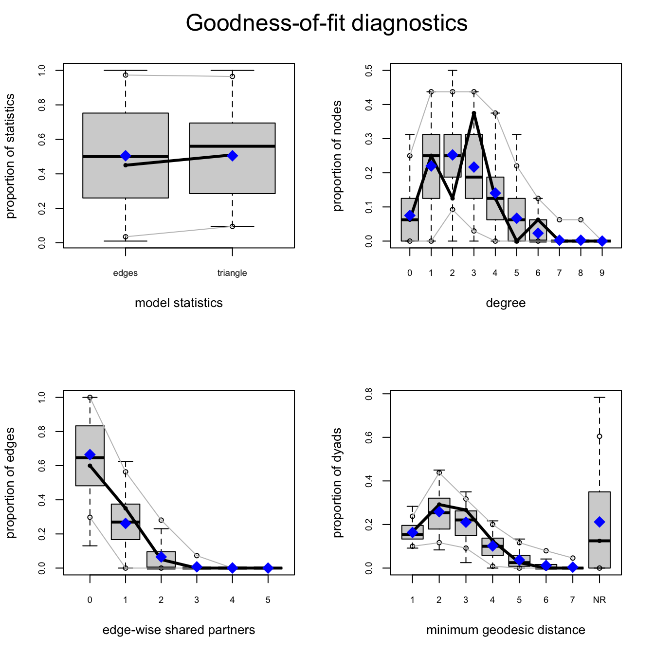
To get an output containing the summary of the gof:
flom_mod2.gof # summary output of gofQ5 How would you interpret the goodness of fit here?
Lazega’s lawyers (from lecture)
We will use the same subset of this network as in the previous lab: we want to check whether or not the partners of the firm more frequently work together with other partners having the same practice. We import the data as a graph object from the networkdata package:
data("law_cowork")We then create an adjacency matrix from the directed graph for the first 36 lawyers in the network corresponding to the partners of the firm (see attribute ‘status’). To test homophily now, we only consider the reciprocal ties so we need to symmetrize the matrix to create and undirected graph:
law_mat_cwdir <- as_adjacency_matrix(law_cowork, sparse = FALSE)
law_mat_cwdir <- law_mat_cwdir[1:36,1:36]
law_mat_cw <- (law_mat_cwdir == t(law_mat_cwdir) & law_mat_cwdir ==1) + 0Next we save the binary attribute ‘practice’ (1 = litigation, 2 = corporate) from the graph object as a vector, which is then in turn converted into a data frame (again only for the first 36 lawyers who are partners):
law_attr.pract <- vertex_attr(law_cowork)$pract[1:36] - 1Since observed attribute values are 1/2, we subtract 1 to get a 0/1 variable which is easier to interpret in an ERGM context.
We create a network object and add the node attribute ‘practice’:
law_net <- as.network(law_mat_cw, directed = FALSE)
law_net %v% "practice" <- law_attr.pract
law_net Network attributes:
vertices = 36
directed = FALSE
hyper = FALSE
loops = FALSE
multiple = FALSE
bipartite = FALSE
total edges= 115
missing edges= 0
non-missing edges= 115
Vertex attribute names:
practice vertex.names
No edge attributesModel 1: homophily and clustering
Estimation
We are interested in running an ERGM with the following statistics (as done during lecture)
nodecov(“practice”)
match(“practice”)
gwesp(decay = 0.693)
Q6 Can you recall what these statistics represent? To run the ERGM:
law_mod1 <- ergm(law_net ~ edges
+ nodecov("practice") + match("practice")
+ gwesp(0.693, fixed = TRUE)
)
summary(law_mod1)Call:
ergm(formula = law_net ~ edges + nodecov("practice") + match("practice") +
gwesp(0.693, fixed = TRUE))
Monte Carlo Maximum Likelihood Results:
Estimate Std. Error MCMC % z value Pr(>|z|)
edges -4.40585 0.32293 0 -13.643 < 1e-04 ***
nodecov.practice 0.17540 0.07822 0 2.242 0.024942 *
nodematch.practice 0.61329 0.17500 0 3.504 0.000458 ***
gwesp.fixed.0.693 1.15219 0.15967 0 7.216 < 1e-04 ***
---
Signif. codes: 0 '***' 0.001 '**' 0.01 '*' 0.05 '.' 0.1 ' ' 1
Null Deviance: 873.4 on 630 degrees of freedom
Residual Deviance: 502.8 on 626 degrees of freedom
AIC: 510.8 BIC: 528.6 (Smaller is better. MC Std. Err. = 0.3076)See lecture slides for the interpretation of these coefficients.
MCMC diagnostics
Check the model by running MCMC diagnostics to observe what is happening with the simulation algorithm:
mcmc.diagnostics(law_mod1, center = TRUE)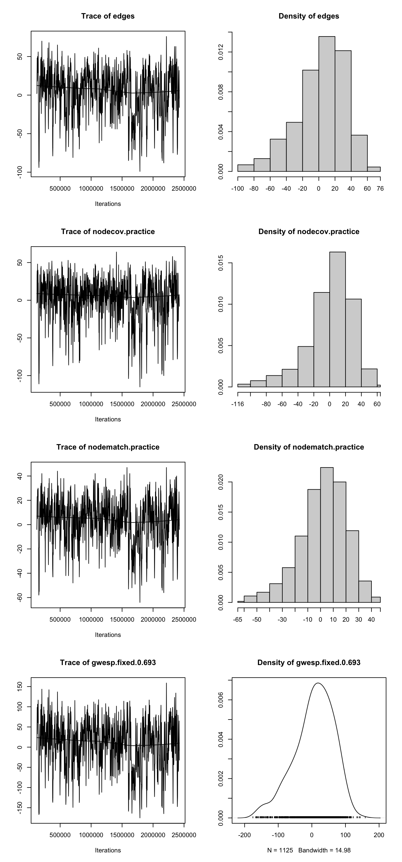
Sample statistics summary:
Iterations = 229376:4489216
Thinning interval = 8192
Number of chains = 1
Sample size per chain = 521
1. Empirical mean and standard deviation for each variable,
plus standard error of the mean:
Mean SD Naive SE Time-series SE
edges 2.873 28.97 1.2692 1.686
nodecov.practice 5.472 26.86 1.1766 1.330
nodematch.practice 1.816 17.76 0.7782 1.105
gwesp.fixed.0.693 6.493 57.22 2.5071 3.240
2. Quantiles for each variable:
2.5% 25% 50% 75% 97.5%
edges -56.0 -15.00 6.00 23.00 53.0
nodecov.practice -59.0 -10.00 10.00 24.00 48.0
nodematch.practice -37.0 -9.00 3.00 14.00 33.0
gwesp.fixed.0.693 -110.6 -30.89 12.37 45.45 108.6
Are sample statistics significantly different from observed?
edges nodecov.practice nodematch.practice gwesp.fixed.0.693
diff. 2.87332054 5.472169e+00 1.8157390 6.49349193
test stat. 1.70443427 4.114483e+00 1.6431992 2.00438393
P-val. 0.08829999 3.880485e-05 0.1003417 0.04502895
(Omni)
diff. NA
test stat. 3.322843e+01
P-val. 1.994933e-06
Sample statistics cross-correlations:
edges nodecov.practice nodematch.practice
edges 1.0000000 0.8698784 0.9464560
nodecov.practice 0.8698784 1.0000000 0.8320838
nodematch.practice 0.9464560 0.8320838 1.0000000
gwesp.fixed.0.693 0.9935680 0.8781753 0.9402085
gwesp.fixed.0.693
edges 0.9935680
nodecov.practice 0.8781753
nodematch.practice 0.9402085
gwesp.fixed.0.693 1.0000000
Sample statistics auto-correlation:
Chain 1
edges nodecov.practice nodematch.practice gwesp.fixed.0.693
Lag 0 1.000000000 1.00000000 1.000000000 1.000000000
Lag 8192 0.264384258 0.19001116 0.253833293 0.243299905
Lag 16384 0.137919062 0.10438774 0.147677955 0.127370433
Lag 24576 -0.005218755 -0.09135989 0.004816156 -0.016619964
Lag 32768 0.007934509 -0.07788227 0.023034765 -0.005065821
Lag 40960 0.055722172 0.04259625 0.063132784 0.044208718
Sample statistics burn-in diagnostic (Geweke):
Chain 1
Fraction in 1st window = 0.1
Fraction in 2nd window = 0.5
edges nodecov.practice nodematch.practice gwesp.fixed.0.693
-0.8457193 -0.7756416 -0.7844341 -0.9158578
Individual P-values (lower = worse):
edges nodecov.practice nodematch.practice gwesp.fixed.0.693
0.3977094 0.4379606 0.4327855 0.3597415
Joint P-value (lower = worse): 0.9021505
Note: MCMC diagnostics shown here are from the last round of
simulation, prior to computation of final parameter estimates.
Because the final estimates are refinements of those used for this
simulation run, these diagnostics may understate model performance.
To directly assess the performance of the final model on in-model
statistics, please use the GOF command: gof(ergmFitObject,
GOF=~model).Q6 Do you see any problems with model degeneracy here? Is the estimation process working as it should?
Goodness of Fit
Goodness of fit can be checked as done earlier:
law_mod1.gof <- gof(law_mod1) # this will produce 4 plots
par(mfrow = c(2, 2)) # figure orientation with 2 rows and 2 columns
plot(law_mod1.gof)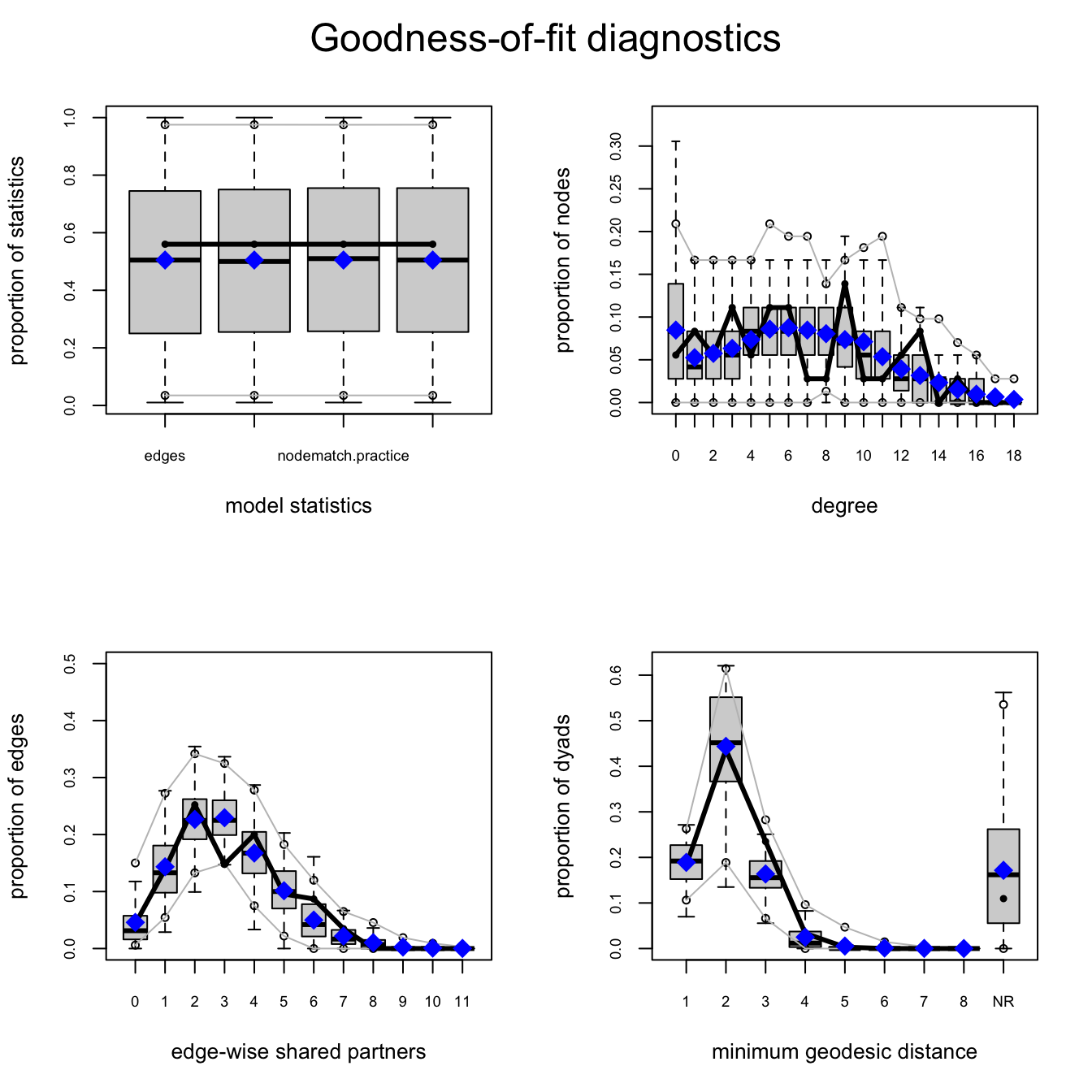
Note that you should not use esp to assess goodness of fit since it was explicitly modeled via the gwesp term in the specified model.
Knecht’s Friendship Network
For the last part, we will fir an ERGM to a directed network to check for reciprocity. We use a friendship network (Knecht,2008) which can be loaded using the networkdata package. You can read about the network by typing ?knecht. Note that the network is longitudinal and observed over four time periods. We will here focus on the last time period. To load the wave 4 data and to visualize it:
data("knecht")
knecht4_g <- knecht[[4]]
knecht4_p <- ggraph(knecht4_g, layout = "stress") +
geom_edge_link(edge_colour = "#666060", end_cap = circle(9,"pt"),
n = 2, edge_width = 0.4, edge_alpha = 1,
arrow = arrow(angle = 15,
length = unit(0.1, "inches"),
ends = "last", type = "closed")) +
geom_node_point(fill = "#000000", colour = "#000000",
size = 7, shape = 21, stroke = 0.9) +
theme_graph() +
theme(legend.position = "none") +
ggtitle("Observed network (wave 4)")
knecht4_p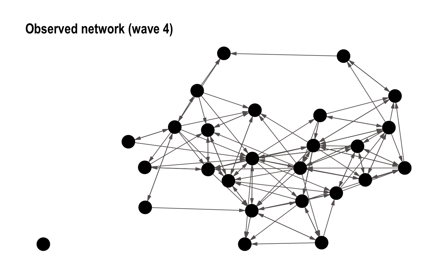
Next we create the network object to fit ERGMs:
# to create network objects
knecht4_net <- asNetwork(knecht[[4]])Model 1: Reciprocity effect
Estimation
knecht4_mod1 <- ergm(knecht4_net ~ edges + mutual)
summary(knecht4_mod1) Call:
ergm(formula = knecht4_net ~ edges + mutual)
Monte Carlo Maximum Likelihood Results:
Estimate Std. Error MCMC % z value Pr(>|z|)
edges -2.1896 0.1579 0 -13.866 <1e-04 ***
mutual 2.4089 0.3401 0 7.084 <1e-04 ***
---
Signif. codes: 0 '***' 0.001 '**' 0.01 '*' 0.05 '.' 0.1 ' ' 1
Null Deviance: 901.1 on 650 degrees of freedom
Residual Deviance: 563.7 on 648 degrees of freedom
AIC: 567.7 BIC: 576.6 (Smaller is better. MC Std. Err. = 0.7431)Q7 How do you interpret these results?
MCMC diagnostics
mcmc.diagnostics(knecht4_mod1)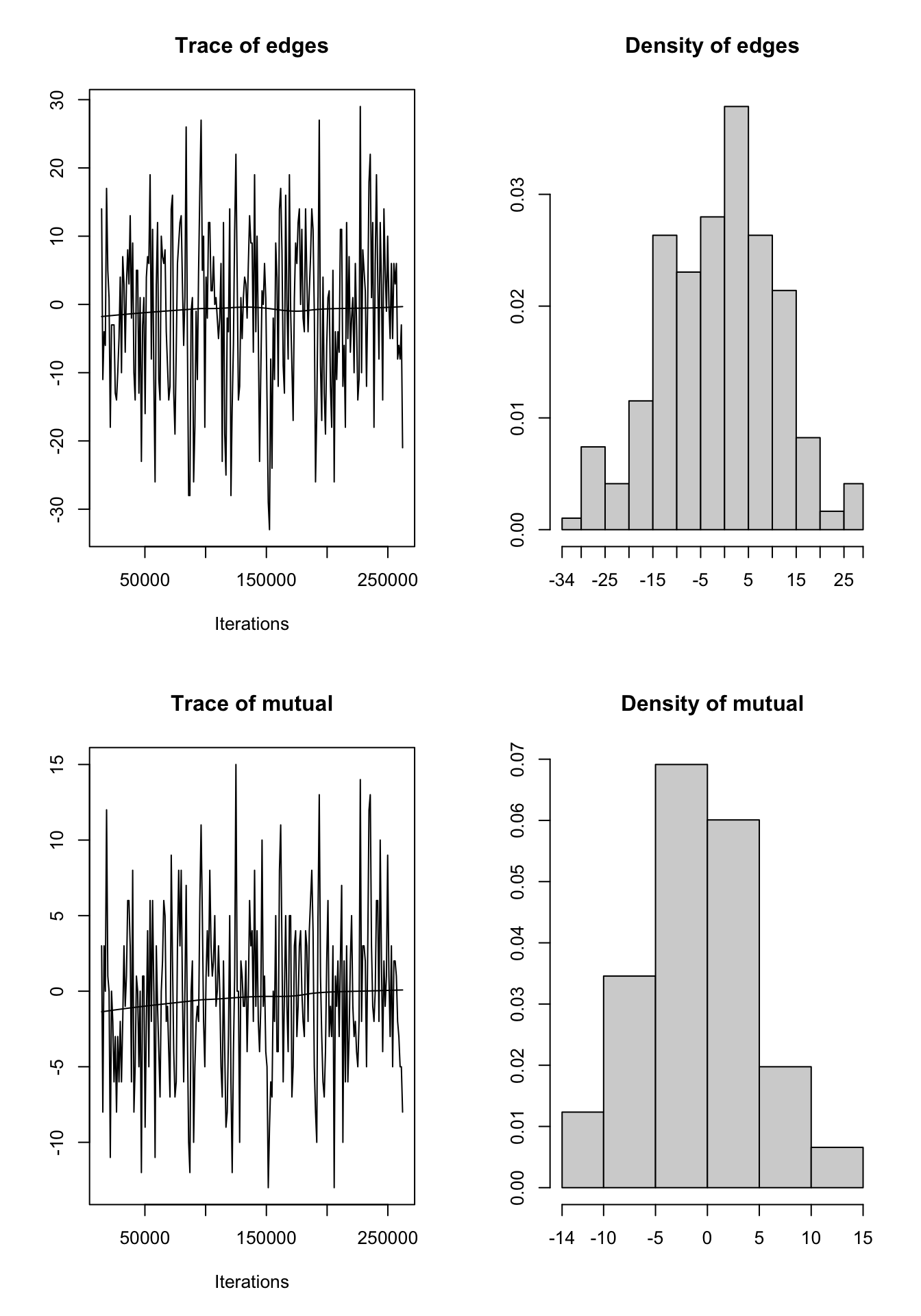
Sample statistics summary:
Iterations = 14336:262144
Thinning interval = 1024
Number of chains = 1
Sample size per chain = 243
1. Empirical mean and standard deviation for each variable,
plus standard error of the mean:
Mean SD Naive SE Time-series SE
edges -0.8519 12.02 0.7712 1.0080
mutual -0.2510 5.58 0.3580 0.4406
2. Quantiles for each variable:
2.5% 25% 50% 75% 97.5%
edges -23.9 -10 -1 6.5 23.95
mutual -11.0 -4 -1 3.0 12.00
Are sample statistics significantly different from observed?
edges mutual (Omni)
diff. -0.8518519 -0.2510288 NA
test stat. -0.8451038 -0.5697862 0.9650027
P-val. 0.3980529 0.5688227 0.6195675
Sample statistics cross-correlations:
edges mutual
edges 1.0000000 0.8485538
mutual 0.8485538 1.0000000
Sample statistics auto-correlation:
Chain 1
edges mutual
Lag 0 1.00000000 1.000000000
Lag 1024 0.25966567 0.202686961
Lag 2048 0.04539234 0.102090560
Lag 3072 -0.02224169 -0.030155517
Lag 4096 -0.10178199 -0.079328021
Lag 5120 -0.04399239 -0.008373088
Sample statistics burn-in diagnostic (Geweke):
Chain 1
Fraction in 1st window = 0.1
Fraction in 2nd window = 0.5
edges mutual
0.03049285 0.29326512
Individual P-values (lower = worse):
edges mutual
0.9756740 0.7693195
Joint P-value (lower = worse): 0.9171878
Note: MCMC diagnostics shown here are from the last round of
simulation, prior to computation of final parameter estimates.
Because the final estimates are refinements of those used for this
simulation run, these diagnostics may understate model performance.
To directly assess the performance of the final model on in-model
statistics, please use the GOF command: gof(ergmFitObject,
GOF=~model).Q8 How do you interpret these results?
Goodness of fit
Note that since we now are considering a directed network, we need to separate in- and out-degree when assessing the goodness of fit:
knecht4_mod1.gof <- gof(knecht4_mod1) # this will produce 4 plots
par(mfrow = c(3,2)) # figure orientation with 2 rows and 2 columns
plot(knecht4_mod1.gof)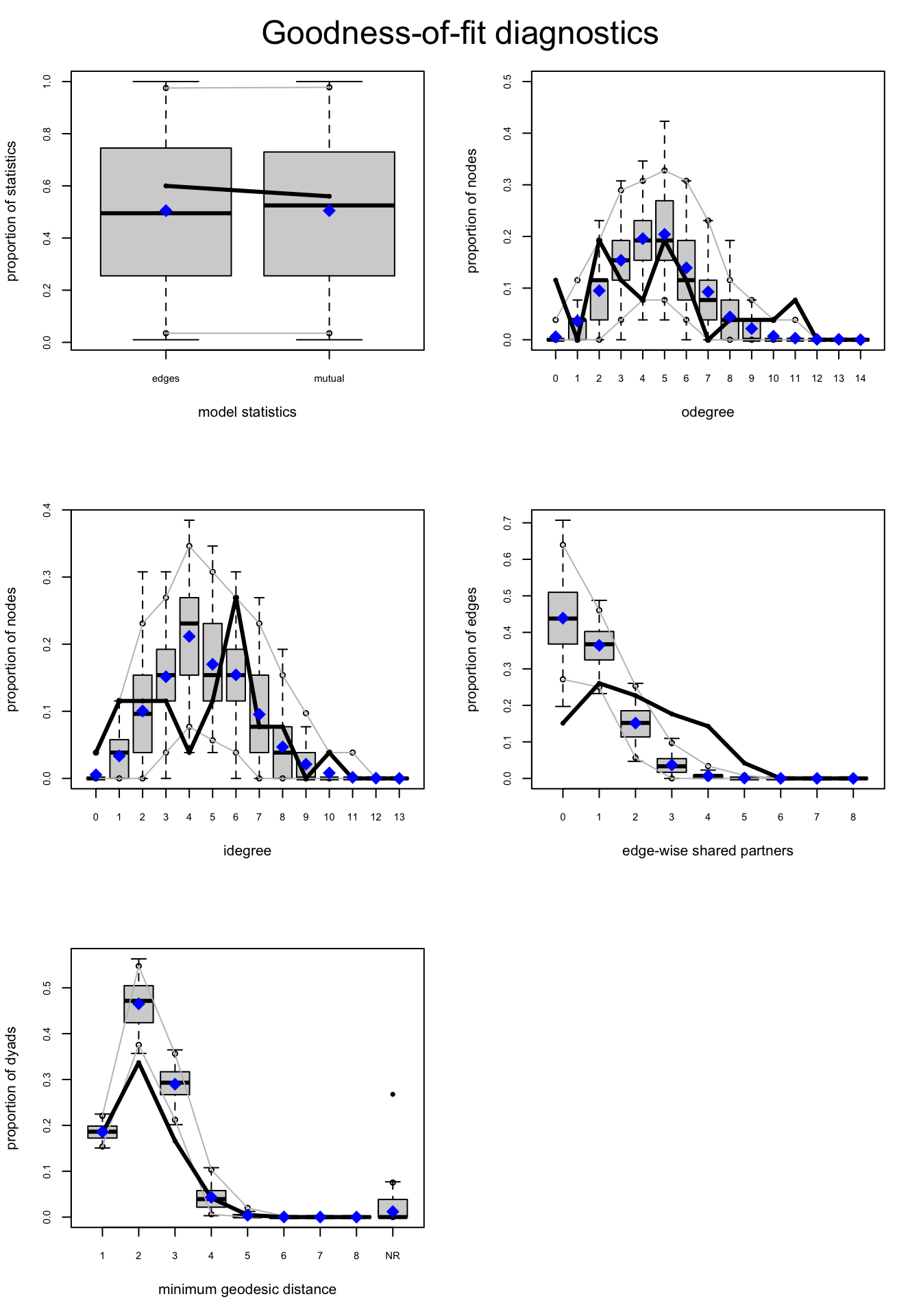
Q9 How do you interpret these results?
Model 2: Modeling Sender, Receiver, Homophily, and Reciprocity Effects
We now include a gender homophily effect to test whether students tend to befriend others of the same gender. We also include separate age-related sender and receiver effects to examine whether older students are more likely to send friendship nominations, receive friendship nominations, or both.
Directed social networks provide information about both who initiates relationships and who receives them. Unlike undirected networks, where ties simply indicate a mutual relationship, directed networks distinguish between outgoing (sent) and incoming (received) ties. This distinction allows ERGMs to model several important social processes simultaneously.
The model below includes terms for sender effects, receiver effects, homophily, and reciprocity:
knecht4_mod2 <- ergm(
knecht4_net ~
edges +
nodeofactor("gender") +
nodeifactor("gender") +
nodematch("gender") +
nodeocov("age") +
nodeicov("age") +
mutual
)
summary(knecht4_mod2)Call:
ergm(formula = knecht4_net ~ edges + nodeofactor("gender") +
nodeifactor("gender") + nodematch("gender") + nodeocov("age") +
nodeicov("age") + mutual)
Monte Carlo Maximum Likelihood Results:
Estimate Std. Error MCMC % z value Pr(>|z|)
edges -3.53128 3.57719 0 -0.987 0.323562
nodeofactor.gender.2 0.90230 0.26822 0 3.364 0.000768 ***
nodeifactor.gender.2 0.07103 0.27180 0 0.261 0.793821
nodematch.gender 1.23632 0.22321 0 5.539 < 1e-04 ***
nodeocov.age -0.01804 0.25072 0 -0.072 0.942638
nodeicov.age 0.04223 0.25163 0 0.168 0.866726
mutual 2.13542 0.37224 0 5.737 < 1e-04 ***
---
Signif. codes: 0 '***' 0.001 '**' 0.01 '*' 0.05 '.' 0.1 ' ' 1
Null Deviance: 901.1 on 650 degrees of freedom
Residual Deviance: 518.2 on 643 degrees of freedom
AIC: 532.2 BIC: 563.5 (Smaller is better. MC Std. Err. = 0.7225)Each model term captures a different mechanism of friendship formation:
| Model Term | Interpretation |
|---|---|
edges |
Estimates the baseline tendency for friendship ties to occur. This functions similarly to the intercept in a logistic regression model. |
nodeofactor("gender") |
Estimates whether students of a particular gender are more or less likely to initiate friendship nominations (a sender or activity effect). |
nodeifactor("gender") |
Estimates whether students of a particular gender are more or less likely to receive friendship nominations (a receiver or popularity effect). |
nodematch("gender") |
Estimates gender homophily, testing whether students are more likely to nominate peers of the same gender than would be expected by chance. |
nodeocov("age") |
Estimates whether older students tend to send more friendship nominations. |
nodeicov("age") |
Estimates whether older students tend to receive more friendship nominations. |
mutual |
Estimates reciprocity, measuring whether friendship nominations are more likely to be reciprocated. |
This specification separates four distinct social processes that contribute to friendship formation:
- Activity effects describe whether some individuals are generally more likely to nominate others.
- Popularity effects describe whether some individuals are more likely to be nominated by others.
- Homophily measures the tendency for individuals with similar characteristics (such as gender) to form relationships.
- Reciprocity measures the tendency for friendship nominations to be mutual.
By modeling these processes simultaneously, the ERGM can determine whether observed friendship patterns are explained by individual characteristics, preferences for similar peers, reciprocal relationships, or a combination of these mechanisms. This provides a richer understanding of the social processes underlying network formation than can be obtained from descriptive network measures alone.
Q10 Run the usual steps of fitting the ERGM (output given below), interpreting the results and checking the estimation algorithm and assessing the goodness of fit. What can you conclude?
summary(knecht4_mod2)Call:
ergm(formula = knecht4_net ~ edges + nodeofactor("gender") +
nodeifactor("gender") + nodematch("gender") + nodeocov("age") +
nodeicov("age") + mutual)
Monte Carlo Maximum Likelihood Results:
Estimate Std. Error MCMC % z value Pr(>|z|)
edges -3.53128 3.57719 0 -0.987 0.323562
nodeofactor.gender.2 0.90230 0.26822 0 3.364 0.000768 ***
nodeifactor.gender.2 0.07103 0.27180 0 0.261 0.793821
nodematch.gender 1.23632 0.22321 0 5.539 < 1e-04 ***
nodeocov.age -0.01804 0.25072 0 -0.072 0.942638
nodeicov.age 0.04223 0.25163 0 0.168 0.866726
mutual 2.13542 0.37224 0 5.737 < 1e-04 ***
---
Signif. codes: 0 '***' 0.001 '**' 0.01 '*' 0.05 '.' 0.1 ' ' 1
Null Deviance: 901.1 on 650 degrees of freedom
Residual Deviance: 518.2 on 643 degrees of freedom
AIC: 532.2 BIC: 563.5 (Smaller is better. MC Std. Err. = 0.7225)Exercises
Exercise 1 Use the undirected cowork network of the lawyer data.
(a) Focus on the attribute ‘gender’ now. Fit an ERGM that potentially could answer whether or not the partners of the firm more frequently work together with other partners of the same gender.
(b) Focus now instead on all 71 lawyers of the data and fit an ERGM that potentially could answer whether or not the partners of the firm more frequently work together with other partners of the firm.
(c) Can you understand why maximum pseudolikelihood estimation (MPLE) is used when only including nodecov() and match() terms?
Exercise 2: Import the data on Kapferer’s Tailors from the package networkdata. You can read about the data by typing ?mine. Note that the data is imported as graph objects so to convert it to a network object, type the following:
mine_net <- asNetwork(mine)Perform the following tasks:
(a) Fit en ERGM with edges and triangles included. How do you interpret the coefficients?
(b) Run MCMC diagnostics on the model in (a). Do you not any problems in the estimation process?
(c) Perform a goodness of fit assessment on the model in (a). What can you conclude?
Exercise 3: Use the directed Knecht friendship networks for this exercise.
(a) We wish to compare the reciprocity effect from wave 1 to wave 4. We fitted the ERGM for wave 4 above. Run the same ERGM for wave 1 and run the usual checks of the fitted model. Can you notice a difference in reciprocity over time?
(b) Run the same comparison as in (a) but also include gender homophily in your model specification. Can you notice a difference in the effects from wave 1 to wave 4?