library(igraph)
library(networkdata)
library(RSiena)Social Network Analysis
Worksheet 11: SAOMs I
Introduction
In this practical we will estimate a Stochastic Actor-Oriented Model (SAOM) using the Teenage Friends and Lifestyle Study.
The data consist of:
- Three waves of friendship nominations among 129 pupils.
- Individual characteristics such as sex.
- Smoking behavior measured at each wave.
The goal is to learn how friendship networks evolve over time and how smoking behavior co-evolves with friendships.
Load packages
Load the data
The dataset contains three friendship networks measured over time.
data("glasgow129")

glasgow_g1 <- glasgow129[[1]]
glasgow_g2 <- glasgow129[[2]]
glasgow_g3 <- glasgow129[[3]]
Prepare the friendship networks
RSiena requires the network to be stored as a three-dimensional array:
- rows = sender
- columns = receiver
- third dimension = observation wave
net1 <- as_adjacency_matrix(glasgow_g1, sparse = FALSE)
net2 <- as_adjacency_matrix(glasgow_g2, sparse = FALSE)
net3 <- as_adjacency_matrix(glasgow_g3, sparse = FALSE)

friendshipArray <- array(
  c(net1, net2, net3),
  dim = c(129,129,3)
)
Model 1: Network dynamics only
We begin with a simple model that explains changes in friendship using only structural network effects.
Creating the dependent network
The friendship network is the dependent variable.
The function sienaDependent() tells RSiena that this network changes over time and should be modelled.
friendship <- sienaDependent(friendshipArray)First we create a Siena data object.
mydata1 <- sienaDataCreate(friendship)Next we create an object that will contain the effects to estimate.
myeff1 <- getEffects(mydata1)Let’s inspect the default effects.
myeff1 effectName include fix test initialValue parm
1 constant friendship rate (period 1) TRUE FALSE FALSE 7.45424 0
2 constant friendship rate (period 2) TRUE FALSE FALSE 6.82927 0
3 outdegree (density) TRUE FALSE FALSE -1.61299 0
4 reciprocity TRUE FALSE FALSE 0.00000 0 Adding structural effects
We now add three common network mechanisms.
myeff1 <- includeEffects(
  myeff1,
  outdegree,
  recip,
  transTrip
)
effectNumber effectName shortName include fix test initialValue
1 15 reciprocity recip TRUE FALSE FALSE 0
2 21 transitive triplets transTrip TRUE FALSE FALSE 0
parm
1 0
2 0 These effects represent:
- Outdegree (density): baseline tendency to create friendships.
- Reciprocity: tendency to reciprocate friendships.
- Transitive triplets: tendency for friends of friends to become friends.
Estimate the model
The estimation algorithm first needs to be specified.
myalgorithm1 <- sienaAlgorithmCreate(
  projname="SAOM1",
  seed=12345
)
If you use this algorithm object, siena07 will create/use an output file SAOM1.txt .Now estimate the model.
result1 <- siena07(
  myalgorithm1,
  data=mydata1,
  effects=myeff1,
  batch=TRUE
)
Start phase 0
theta: -1.61  0.00  0.00

Start phase 1
Phase 1 Iteration 1 Progress: 0%
Phase 1 Iteration 2 Progress: 0%
Phase 1 Iteration 3 Progress: 0%
Phase 1 Iteration 4 Progress: 0%
Phase 1 Iteration 5 Progress: 0%
Phase 1 Iteration 10 Progress: 0%
Phase 1 Iteration 15 Progress: 1%
Phase 1 Iteration 20 Progress: 1%
Phase 1 Iteration 25 Progress: 1%
Phase 1 Iteration 30 Progress: 1%
Phase 1 Iteration 35 Progress: 1%
Phase 1 Iteration 40 Progress: 2%
Phase 1 Iteration 45 Progress: 2%
Phase 1 Iteration 50 Progress: 2%
theta: -1.722  0.282  0.113

Start phase 2.1
Phase 2 Subphase 1 Iteration 1 Progress: 8%
Phase 2 Subphase 1 Iteration 2 Progress: 8%
theta -1.755  0.366  0.147
ac 0.924 1.116 1.074
Phase 2 Subphase 1 Iteration 3 Progress: 8%
Phase 2 Subphase 1 Iteration 4 Progress: 8%
theta -1.862  0.627  0.254
ac 0.868 1.153 1.144
Phase 2 Subphase 1 Iteration 5 Progress: 8%
Phase 2 Subphase 1 Iteration 6 Progress: 8%
theta -1.987  0.921  0.372
ac 0.886 1.159 1.175
Phase 2 Subphase 1 Iteration 7 Progress: 8%
Phase 2 Subphase 1 Iteration 8 Progress: 8%
theta -2.129  1.252  0.475
ac 0.931 1.170 1.153
Phase 2 Subphase 1 Iteration 9 Progress: 8%
Phase 2 Subphase 1 Iteration 10 Progress: 8%
theta -2.246  1.541  0.486
ac 0.994 1.174 1.277
theta -2.619  2.144  0.455
ac  0.490  0.115 -0.367
theta: -2.619  2.144  0.455

Start phase 2.2
Phase 2 Subphase 2 Iteration 1 Progress: 16%
Phase 2 Subphase 2 Iteration 2 Progress: 16%
Phase 2 Subphase 2 Iteration 3 Progress: 16%
Phase 2 Subphase 2 Iteration 4 Progress: 16%
Phase 2 Subphase 2 Iteration 5 Progress: 16%
Phase 2 Subphase 2 Iteration 6 Progress: 16%
Phase 2 Subphase 2 Iteration 7 Progress: 16%
Phase 2 Subphase 2 Iteration 8 Progress: 16%
Phase 2 Subphase 2 Iteration 9 Progress: 16%
Phase 2 Subphase 2 Iteration 10 Progress: 16%
theta -2.628  2.172  0.456
ac -0.365 -0.513 -0.553
theta: -2.628  2.172  0.456

Start phase 2.3
Phase 2 Subphase 3 Iteration 1 Progress: 26%
Phase 2 Subphase 3 Iteration 2 Progress: 26%
Phase 2 Subphase 3 Iteration 3 Progress: 26%
Phase 2 Subphase 3 Iteration 4 Progress: 26%
Phase 2 Subphase 3 Iteration 5 Progress: 26%
Phase 2 Subphase 3 Iteration 6 Progress: 26%
Phase 2 Subphase 3 Iteration 7 Progress: 26%
Phase 2 Subphase 3 Iteration 8 Progress: 26%
Phase 2 Subphase 3 Iteration 9 Progress: 26%
Phase 2 Subphase 3 Iteration 10 Progress: 26%
theta -2.638  2.183  0.458
ac -0.0356 -0.1058 -0.0708
theta: -2.638  2.183  0.458

Start phase 2.4
Phase 2 Subphase 4 Iteration 1 Progress: 40%
Phase 2 Subphase 4 Iteration 2 Progress: 40%
Phase 2 Subphase 4 Iteration 3 Progress: 40%
Phase 2 Subphase 4 Iteration 4 Progress: 40%
Phase 2 Subphase 4 Iteration 5 Progress: 40%
Phase 2 Subphase 4 Iteration 6 Progress: 40%
Phase 2 Subphase 4 Iteration 7 Progress: 40%
Phase 2 Subphase 4 Iteration 8 Progress: 40%
Phase 2 Subphase 4 Iteration 9 Progress: 40%
Phase 2 Subphase 4 Iteration 10 Progress: 40%
theta -2.639  2.177  0.462
ac -0.0717 -0.1472 -0.0711
theta: -2.639  2.177  0.462

Start phase 3
Phase 3 Iteration 500 Progress 81%
Phase 3 Iteration 1000 Progress 100%
Display the results.
summary(result1)Estimates, standard errors and convergence t-ratios
Estimate Standard Convergence
Error t-ratio
Rate parameters:
0.1 Rate parameter period 1 10.6606 ( 1.0645 )
0.2 Rate parameter period 2 8.7846 ( 0.8342 )
Other parameters:
1. eval outdegree (density) -2.6386 ( 0.0422 ) 0.0671
2. eval reciprocity 2.1774 ( 0.0932 ) 0.0688
3. eval transitive triplets 0.4622 ( 0.0294 ) 0.1123
Overall maximum convergence ratio: 0.1188
Total of 1894 iteration steps.
Covariance matrix of estimates (correlations below diagonal)
0.002 -0.002 -0.001
-0.400 0.009 -0.001
-0.453 -0.292 0.001
Derivative matrix of expected statistics X by parameters:
1365.263 870.751 2440.256
475.244 498.340 1266.413
1958.805 1673.528 9163.139
Covariance matrix of X (correlations below diagonal):
2065.855 1629.841 6964.869
0.899 1592.616 6759.701
0.732 0.809 43788.925Model 2: Adding actor covariates
Next we investigate whether friendships depend on:
- sex
- smoking
Sex
The sex variable does not change over time.
Therefore it is entered as a constant covariate.
sex <- ifelse(
  V(glasgow_g2)$sex.F=="F",
  1,
  0
)

sexCov <- coCovar(sex)
Smoking
Smoking is observed at every wave.
We therefore create a changing covariate.
smoke <- cbind(
  as.numeric(V(glasgow_g1)$tobacco),
  as.numeric(V(glasgow_g2)$tobacco),
  as.numeric(V(glasgow_g3)$tobacco)
)

smokeCov <- varCovar(smoke)
Create the new Siena data object
mydata2 <- sienaDataCreate(
  friendship,
  sexCov,
  smokeCov
)
myeff2 <- getEffects(mydata2)Add covariate effects
For each covariate we estimate three effects.
myeff2 <- includeEffects(
  myeff2,
  egoX,
  altX,
  simX,
  interaction1="sexCov"
)
effectNumber effectName shortName include fix test initialValue
1 264 sexCov alter altX TRUE FALSE FALSE 0
2 279 sexCov ego egoX TRUE FALSE FALSE 0
3 325 sexCov similarity simX TRUE FALSE FALSE 0
parm
1 0
2 0
3 0 myeff2 <- includeEffects(
myeff2,
egoX,
altX,
simX,
interaction1="smokeCov"
) effectNumber effectName shortName include fix test initialValue
1 448 smokeCov alter altX TRUE FALSE FALSE 0
2 463 smokeCov ego egoX TRUE FALSE FALSE 0
3 509 smokeCov similarity simX TRUE FALSE FALSE 0
parm
1 0
2 0
3 0 These correspond to:
- ego effect: Does this type of actor nominate more friends?
- alter effect: Are actors with this characteristic more popular?
- similarity effect: Do similar actors become friends?
Estimate Model 2
myalgorithm2 <- sienaAlgorithmCreate(
  projname="SAOM2",
  seed=12345
)
If you use this algorithm object, siena07 will create/use an output file SAOM2.txt .result2 <- siena07(
myalgorithm2,
data=mydata2,
effects=myeff2,
batch=TRUE
)
Start phase 0
theta: -1.61  0.00  0.00  0.00  0.00  0.00  0.00  0.00

Start phase 1
Phase 1 Iteration 1 Progress: 0%
Phase 1 Iteration 2 Progress: 0%
Phase 1 Iteration 3 Progress: 0%
Phase 1 Iteration 4 Progress: 0%
Phase 1 Iteration 5 Progress: 0%
Phase 1 Iteration 10 Progress: 0%
Phase 1 Iteration 15 Progress: 0%
Phase 1 Iteration 20 Progress: 1%
Phase 1 Iteration 25 Progress: 1%
Phase 1 Iteration 30 Progress: 1%
Phase 1 Iteration 35 Progress: 1%
Phase 1 Iteration 40 Progress: 1%
Phase 1 Iteration 45 Progress: 1%
Phase 1 Iteration 50 Progress: 2%
theta: -1.68133  0.32727 -0.02170  0.01601  0.07934  0.00680  0.00077  0.08581

Start phase 2.1
Phase 2 Subphase 1 Iteration 1 Progress: 14%
Phase 2 Subphase 1 Iteration 2 Progress: 14%
theta -1.725465  0.534183 -0.033884  0.026220  0.130621  0.009735  0.000769  0.135120
ac 0.920 1.134 1.080 0.829 1.181 9.733 1.552 1.397
Phase 2 Subphase 1 Iteration 3 Progress: 14%
Phase 2 Subphase 1 Iteration 4 Progress: 14%
theta -1.87129  1.18486 -0.07152  0.05461  0.28941  0.02781  0.00599  0.28414
ac 0.935 1.181 0.924 1.052 1.228 5.969 1.538 1.473
Phase 2 Subphase 1 Iteration 5 Progress: 14%
Phase 2 Subphase 1 Iteration 6 Progress: 14%
theta -2.0539  1.8856 -0.0936  0.0785  0.4710  0.0412  0.0152  0.3994
ac 0.962 1.192 1.014 1.158 1.225 1.812 1.412 1.484
Phase 2 Subphase 1 Iteration 7 Progress: 14%
Phase 2 Subphase 1 Iteration 8 Progress: 14%
theta -2.2518  2.3224 -0.0871  0.1050  0.6927  0.0409  0.0346  0.4577
ac 0.986 1.180 1.188 1.216 1.213 1.626 1.405 1.375
Phase 2 Subphase 1 Iteration 9 Progress: 14%
Phase 2 Subphase 1 Iteration 10 Progress: 14%
theta -2.4044  2.4850 -0.0592  0.1109  0.8201  0.0377  0.0453  0.4276
ac 1.00 1.18 1.41 1.22 1.19 1.84 1.40 1.38
theta -2.63e+00  2.48e+00 -1.28e-01  1.77e-01  9.89e-01  5.62e-02 -9.63e-05  4.23e-01
ac 0.8588 0.9866 0.0467 0.0214 0.7584 0.0682 0.0831 0.0376
theta: -2.63e+00  2.48e+00 -1.28e-01  1.77e-01  9.89e-01  5.62e-02 -9.63e-05  4.23e-01

Start phase 2.2
Phase 2 Subphase 2 Iteration 1 Progress: 21%
Phase 2 Subphase 2 Iteration 2 Progress: 22%
Phase 2 Subphase 2 Iteration 3 Progress: 22%
Phase 2 Subphase 2 Iteration 4 Progress: 22%
Phase 2 Subphase 2 Iteration 5 Progress: 22%
Phase 2 Subphase 2 Iteration 6 Progress: 22%
Phase 2 Subphase 2 Iteration 7 Progress: 22%
Phase 2 Subphase 2 Iteration 8 Progress: 22%
Phase 2 Subphase 2 Iteration 9 Progress: 22%
Phase 2 Subphase 2 Iteration 10 Progress: 22%
theta -2.63747  2.50132 -0.13555  0.18807  0.99309  0.05502  0.00103  0.42691
ac  0.09984 -0.08123 -0.00364 -0.05184  0.10793 -0.05866 -0.13339 -0.07239
theta: -2.63747  2.50132 -0.13555  0.18807  0.99309  0.05502  0.00103  0.42691

Start phase 2.3
Phase 2 Subphase 3 Iteration 1 Progress: 31%
Phase 2 Subphase 3 Iteration 2 Progress: 31%
Phase 2 Subphase 3 Iteration 3 Progress: 31%
Phase 2 Subphase 3 Iteration 4 Progress: 31%
Phase 2 Subphase 3 Iteration 5 Progress: 31%
Phase 2 Subphase 3 Iteration 6 Progress: 31%
Phase 2 Subphase 3 Iteration 7 Progress: 31%
Phase 2 Subphase 3 Iteration 8 Progress: 31%
Phase 2 Subphase 3 Iteration 9 Progress: 31%
Phase 2 Subphase 3 Iteration 10 Progress: 31%
theta -2.63525  2.49942 -0.12682  0.17269  0.98763  0.06401  0.00105  0.43755
ac -0.01540 -0.06028  0.09565  0.08035  0.01697  0.00189 -0.08490 -0.13846
theta: -2.63525  2.49942 -0.12682  0.17269  0.98763  0.06401  0.00105  0.43755

Start phase 2.4
Phase 2 Subphase 4 Iteration 1 Progress: 44%
Phase 2 Subphase 4 Iteration 2 Progress: 44%
Phase 2 Subphase 4 Iteration 3 Progress: 44%
Phase 2 Subphase 4 Iteration 4 Progress: 44%
Phase 2 Subphase 4 Iteration 5 Progress: 44%
Phase 2 Subphase 4 Iteration 6 Progress: 44%
Phase 2 Subphase 4 Iteration 7 Progress: 44%
Phase 2 Subphase 4 Iteration 8 Progress: 44%
Phase 2 Subphase 4 Iteration 9 Progress: 44%
Phase 2 Subphase 4 Iteration 10 Progress: 44%
theta -2.62789  2.49425 -0.12769  0.17550  0.98194  0.05515  0.00273  0.42459
ac -0.00709  0.11036 -0.07095  0.02080 -0.05686 -0.01517 -0.06179 -0.01688
theta: -2.62789  2.49425 -0.12769  0.17550  0.98194  0.05515  0.00273  0.42459

Start phase 3
Phase 3 Iteration 500 Progress 84%
Phase 3 Iteration 1000 Progress 100%summary(result2)Estimates, standard errors and convergence t-ratios
Estimate Standard Convergence
Error t-ratio
Rate parameters:
0.1 Rate parameter period 1 8.8650 ( 0.7610 )
0.2 Rate parameter period 2 7.5790 ( 0.5836 )
Other parameters:
1. eval outdegree (density) -2.6279 ( 0.0477 ) 0.0140
2. eval reciprocity 2.4942 ( 0.0835 ) -0.0103
3. eval sexCov alter -0.1277 ( 0.0946 ) 0.0058
4. eval sexCov ego 0.1755 ( 0.0954 ) 0.0572
5. eval sexCov similarity 0.9819 ( 0.0856 ) -0.0205
6. eval smokeCov alter 0.0552 ( 0.0637 ) -0.0144
7. eval smokeCov ego 0.0027 ( 0.0675 ) 0.0613
8. eval smokeCov similarity 0.4246 ( 0.1193 ) -0.0230
Overall maximum convergence ratio: 0.1306
Total of 2803 iteration steps.
Covariance matrix of estimates (correlations below diagonal)
0.002 -0.002 0.001 -0.001 -0.002 0.000 0.000 -0.001
-0.437 0.007 -0.001 0.001 0.000 0.000 0.000 -0.001
0.207 -0.071 0.009 -0.007 -0.002 0.000 0.000 0.001
-0.220 0.073 -0.724 0.009 0.002 0.000 -0.001 -0.001
-0.566 -0.059 -0.206 0.256 0.007 0.000 0.000 0.000
-0.029 -0.061 -0.063 -0.026 0.041 0.004 0.000 0.003
0.024 -0.052 -0.020 -0.134 0.005 -0.074 0.005 0.004
-0.105 -0.086 0.051 -0.053 -0.024 0.437 0.444 0.014
Derivative matrix of expected statistics X by parameters:
886.020 550.999 -39.179 -19.293 326.879 -63.568 -73.563 91.098
305.167 384.190 -6.474 -5.057 125.179 -18.767 -20.962 38.533
-35.182 -11.610 222.483 173.328 -12.164 58.385 60.186 -29.692
-18.794 -18.768 174.248 216.672 -27.408 54.193 61.163 -23.835
323.766 224.861 -13.206 -25.789 232.628 -26.874 -29.579 33.433
-63.515 -37.631 65.918 52.678 -21.790 294.414 142.499 -103.710
-78.885 -45.105 59.313 70.799 -28.159 137.432 277.757 -101.648
97.076 73.663 -32.906 -33.076 39.056 -104.795 -100.765 115.947
Covariance matrix of X (correlations below diagonal):
769.131 564.071 -19.450 -6.342 308.042 -50.363 -55.530 80.344
0.790 663.309 -5.170 -2.196 245.967 -38.650 -37.269 72.746
-0.051 -0.015 190.808 155.126 -6.996 51.392 42.141 -21.379
-0.017 -0.006 0.835 180.717 -12.623 42.802 48.042 -21.352
0.766 0.659 -0.035 -0.065 210.301 -10.160 -12.915 28.810
-0.118 -0.097 0.241 0.207 -0.045 237.445 133.989 -86.320
-0.133 -0.096 0.203 0.238 -0.059 0.578 226.386 -81.709
0.294 0.287 -0.157 -0.161 0.202 -0.568 -0.551 97.158Model 3: Co-evolution of friendship and smoking
So far smoking has only been treated as a covariate.
Now we allow smoking itself to change over time.
We therefore model two dependent variables simultaneously:
- friendship
- smoking behavior
smoking <- sienaDependent(
  smoke,
  type="behavior"
)
Create the co-evolution dataset
mydata3 <- sienaDataCreate(
  friendship,
  smoking,
  sexCov
)

myeff3 <- getEffects(mydata3)
Friendship dynamics
We include the same structural effects as before.
myeff3 <- includeEffects(
  myeff3,
  outdegree,
  recip,
  transTrip,
  name="friendship"
)
effectNumber effectName shortName include fix test initialValue
1 17 reciprocity recip TRUE FALSE FALSE 0
2 23 transitive triplets transTrip TRUE FALSE FALSE 0
parm
1 0
2 0 Behavior dynamics
We now model changes in smoking.
myeff3 <- includeEffects(
  myeff3,
  linear,
  quad,
  name="smoking"
)
effectNumber effectName shortName include fix test
1 689 smoking linear shape linear TRUE FALSE FALSE
2 692 smoking quadratic shape quad TRUE FALSE FALSE
initialValue parm
1 -0.58955 0
2 0.00000 0 The behavioral objective function now estimates:
- Linear shape: Is higher smoking generally more or less attractive?
- Quadratic shape: Are moderate or extreme smoking levels preferred?
Estimate the co-evolution model
myalgorithm3 <- sienaAlgorithmCreate(
  projname="SAOM3",
  seed=12
)
If you use this algorithm object, siena07 will create/use an output file SAOM3.txt .result3 <- siena07(
myalgorithm3,
data = mydata3,
effects = myeff3,
batch = TRUE,
returnDeps = TRUE
)
Start phase 0
theta:  7.454  6.829 -1.613  0.000  0.000  0.472  0.423 -0.590  0.000  0.000

Start phase 1
Phase 1 Iteration 1 Progress: 0%
Phase 1 Iteration 2 Progress: 0%
Phase 1 Iteration 3 Progress: 0%
Phase 1 Iteration 4 Progress: 0%
Phase 1 Iteration 5 Progress: 0%
Phase 1 Iteration 10 Progress: 0%
Phase 1 Iteration 15 Progress: 0%
Phase 1 Iteration 20 Progress: 1%
Phase 1 Iteration 25 Progress: 1%
Phase 1 Iteration 30 Progress: 1%
Phase 1 Iteration 35 Progress: 1%
Phase 1 Iteration 40 Progress: 1%
Phase 1 Iteration 45 Progress: 1%
Phase 1 Iteration 50 Progress: 1%
theta:  7.7352  6.5283 -1.7148  0.2187  0.1403  0.4609  0.4982 -0.6127 -0.0482  1.0000

Start phase 2.1
Phase 2 Subphase 1 Iteration 1 Progress: 16%
Phase 2 Subphase 1 Iteration 2 Progress: 16%
theta  7.8490  6.4278 -1.7661  0.3228  0.2086  0.4620  0.5331 -0.6109 -0.0659  1.4482
ac 2.029 1.528 0.995 1.108 1.138 0.885 1.617 1.199 1.124 1.088
Phase 2 Subphase 1 Iteration 3 Progress: 16%
Phase 2 Subphase 1 Iteration 4 Progress: 16%
theta  8.3692  6.3065 -1.9346  0.6814  0.4121  0.4802  0.6411 -0.6376 -0.0539  3.0664
ac 1.431 1.505 0.910 1.167 1.193 0.697 0.548 0.859 1.061 1.306
Phase 2 Subphase 1 Iteration 5 Progress: 16%
Phase 2 Subphase 1 Iteration 6 Progress: 16%
theta  8.720  6.728 -2.113  1.156  0.500  0.573  0.757 -0.814  0.360  4.764
ac 1.400 1.254 1.030 1.172 1.246 0.732 0.549 0.958 1.103 1.339
Phase 2 Subphase 1 Iteration 7 Progress: 16%
Phase 2 Subphase 1 Iteration 8 Progress: 16%
theta  8.664  7.133 -2.255  1.579  0.449  0.791  0.860 -1.252  1.122  6.240
ac 1.446 1.227 1.097 1.169 1.331 0.774 0.364 0.667 1.123 1.254
Phase 2 Subphase 1 Iteration 9 Progress: 16%
Phase 2 Subphase 1 Iteration 10 Progress: 16%
theta  8.849  7.598 -2.390  1.934  0.412  0.901  0.949 -1.812  1.675  6.596
ac 1.420 1.113 1.130 1.162 1.139 0.733 0.449 0.726 1.081 1.203
theta 10.229  8.570 -2.640  2.187  0.453 13.231  9.742 -7.707  6.706  3.856
ac  0.361  0.183  0.244 -0.177 -0.599  0.664  0.790  0.298  0.384  0.438
theta: 10.229  8.570 -2.640  2.187  0.453 13.231  9.742 -7.707  6.706  3.856

Start phase 2.2
Phase 2 Subphase 2 Iteration 1 Progress: 23%
Phase 2 Subphase 2 Iteration 2 Progress: 23%
Phase 2 Subphase 2 Iteration 3 Progress: 23%
Phase 2 Subphase 2 Iteration 4 Progress: 23%
Phase 2 Subphase 2 Iteration 5 Progress: 23%
Phase 2 Subphase 2 Iteration 6 Progress: 23%
Phase 2 Subphase 2 Iteration 7 Progress: 23%
Phase 2 Subphase 2 Iteration 8 Progress: 23%
Phase 2 Subphase 2 Iteration 9 Progress: 23%
Phase 2 Subphase 2 Iteration 10 Progress: 23%
Phase 2 Subphase 2 Iteration 1 Progress: 23%
Phase 2 Subphase 2 Iteration 2 Progress: 23%
Phase 2 Subphase 2 Iteration 3 Progress: 23%
Phase 2 Subphase 2 Iteration 4 Progress: 24%
Phase 2 Subphase 2 Iteration 5 Progress: 24%
Phase 2 Subphase 2 Iteration 6 Progress: 24%
Phase 2 Subphase 2 Iteration 7 Progress: 24%
Phase 2 Subphase 2 Iteration 8 Progress: 24%
Phase 2 Subphase 2 Iteration 9 Progress: 24%
Phase 2 Subphase 2 Iteration 10 Progress: 24%
theta 10.781  8.738 -2.632  2.177  0.458  4.939  4.044 -4.912  4.268  2.721
ac  0.4096  0.0194 -0.2234 -0.3822 -0.3763  0.6583  0.7999 -0.1842 -0.3424  0.2468
theta: 10.781  8.738 -2.632  2.177  0.458  4.939  4.044 -4.912  4.268  2.721

Start phase 2.3
Phase 2 Subphase 3 Iteration 1 Progress: 32%
Phase 2 Subphase 3 Iteration 2 Progress: 32%
Phase 2 Subphase 3 Iteration 3 Progress: 32%
Phase 2 Subphase 3 Iteration 4 Progress: 32%
Phase 2 Subphase 3 Iteration 5 Progress: 32%
Phase 2 Subphase 3 Iteration 6 Progress: 32%
Phase 2 Subphase 3 Iteration 7 Progress: 32%
Phase 2 Subphase 3 Iteration 8 Progress: 32%
Phase 2 Subphase 3 Iteration 9 Progress: 32%
Phase 2 Subphase 3 Iteration 10 Progress: 32%
theta 10.876  8.830 -2.625  2.162  0.457  4.898  4.239 -3.506  2.709  1.768
ac  0.1660 -0.0145 -0.0159 -0.1582 -0.1314  0.4496  0.5568  0.1050 -0.1605  0.1295
theta: 10.876  8.830 -2.625  2.162  0.457  4.898  4.239 -3.506  2.709  1.768

Start phase 2.4
Phase 2 Subphase 4 Iteration 1 Progress: 46%
Phase 2 Subphase 4 Iteration 2 Progress: 46%
Phase 2 Subphase 4 Iteration 3 Progress: 46%
Phase 2 Subphase 4 Iteration 4 Progress: 46%
Phase 2 Subphase 4 Iteration 5 Progress: 46%
Phase 2 Subphase 4 Iteration 6 Progress: 46%
Phase 2 Subphase 4 Iteration 7 Progress: 46%
Phase 2 Subphase 4 Iteration 8 Progress: 46%
Phase 2 Subphase 4 Iteration 9 Progress: 46%
Phase 2 Subphase 4 Iteration 10 Progress: 46%
theta 10.652  8.719 -2.630  2.170  0.458  4.237  3.522 -3.824  3.057  2.013
ac  0.10618  0.01752 -0.03423 -0.12617 -0.16822  0.28303  0.36789  0.08696  0.00477  0.04506
theta: 10.652  8.719 -2.630  2.170  0.458  4.237  3.522 -3.824  3.057  2.013

Start phase 3
Phase 3 Iteration 500 Progress 85%
Phase 3 Iteration 1000 Progress 100%summary(result3)Estimates, standard errors and convergence t-ratios
Estimate Standard Convergence
Error t-ratio
Network Dynamics
1. rate constant friendship rate (period 1) 10.6525 ( 1.0666 ) -0.0800
2. rate constant friendship rate (period 2) 8.7185 ( 0.8924 ) -0.1003
3. eval outdegree (density) -2.6301 ( 0.0416 ) 0.0233
4. eval reciprocity 2.1696 ( 0.0925 ) 0.0112
5. eval transitive triplets 0.4581 ( 0.0287 ) -0.0117
Behavior Dynamics
6. rate rate smoking (period 1) 4.2365 ( 1.4498 ) -0.2653
7. rate rate smoking (period 2) 3.5222 ( 1.0394 ) -0.3636
8. eval smoking linear shape -3.8244 ( 0.4564 ) 0.0583
9. eval smoking quadratic shape 3.0574 ( 0.4022 ) 0.1809
10. eval smoking average alter 2.0130 ( 0.8836 ) 0.2322
Overall maximum convergence ratio: 0.9568
Total of 3126 iteration steps.
Covariance matrix of estimates (correlations below diagonal)
1.138 -0.131 0.008 -0.016 -0.002 0.514 0.102 -0.047 0.034 -0.072
-0.138 0.796 0.000 -0.008 0.003 0.026 0.117 -0.042 0.033 0.041
0.191 -0.012 0.002 -0.002 -0.001 0.010 0.000 -0.001 0.000 0.002
-0.165 -0.102 -0.396 0.009 -0.001 -0.022 0.004 0.002 -0.001 -0.006
-0.079 0.122 -0.437 -0.309 0.001 0.000 0.000 0.000 0.001 0.000
0.333 0.020 0.166 -0.161 0.000 2.102 0.128 -0.073 0.067 -0.227
0.092 0.126 -0.001 0.042 0.013 0.085 1.080 -0.172 0.120 -0.289
-0.096 -0.103 -0.041 0.058 -0.033 -0.111 -0.362 0.208 -0.170 -0.183
0.080 0.093 0.013 -0.028 0.056 0.115 0.288 -0.926 0.162 0.143
-0.077 0.052 0.060 -0.071 0.018 -0.177 -0.315 -0.453 0.403 0.781
Derivative matrix of expected statistics X by parameters:
18.078 0.000 2.134 3.622 26.589 1.151 0.000 0.803 0.685 -0.052
0.000 18.873 0.918 2.076 8.729 0.000 0.007 -0.333 -0.475 -1.420
174.590 162.420 1314.240 829.488 2687.800 -21.744 -9.477 -17.482 -20.673 -9.855
35.160 11.272 460.085 484.602 1206.157 -4.031 -10.005 -14.205 -16.763 -2.588
293.847 162.914 1966.573 1669.618 9760.987 -22.797 -24.881 -50.373 -66.690 -20.074
-6.615 0.000 -1.301 0.647 -4.380 3.405 0.000 1.474 2.664 1.209
0.000 -3.877 -4.144 -3.641 -10.333 0.000 8.896 7.757 9.308 5.098
-4.904 -1.689 -17.909 -15.520 -83.718 24.689 24.570 79.219 90.217 35.575
-3.227 -0.933 -20.261 -20.206 -107.511 16.742 11.330 69.094 85.404 32.026
-1.184 -1.407 -4.238 -1.795 -15.960 3.930 7.330 10.860 11.744 16.087
Covariance matrix of X (correlations below diagonal):
382.977 -5.646 262.180 158.533 1267.447 -6.099 4.370 -4.038 -7.862 -5.900
-0.016 322.672 210.522 108.395 911.495 3.181 -4.047 -3.075 -3.444 -7.140
0.305 0.267 1929.418 1512.375 7156.425 -13.647 -16.774 -26.688 -35.665 -16.551
0.212 0.158 0.903 1453.911 6500.039 -5.595 -19.525 -23.697 -33.361 -15.510
0.301 0.236 0.758 0.793 46185.505 -47.038 -67.020 -162.950 -224.604 -154.132
-0.047 0.027 -0.047 -0.022 -0.033 43.901 -0.047 46.116 52.171 18.936
0.032 -0.032 -0.055 -0.074 -0.045 -0.001 48.390 45.909 51.314 29.636
-0.017 -0.014 -0.051 -0.052 -0.064 0.587 0.557 140.630 162.241 78.327
-0.029 -0.014 -0.058 -0.062 -0.074 0.560 0.525 0.973 197.657 96.033
-0.026 -0.034 -0.033 -0.035 -0.062 0.247 0.368 0.571 0.590 133.837
Important
To use sienaGOF()which we do in the next seection, the model must be estimated with returnDeps = TRUE, so that RSiena stores the simulated dependent variables needed for the goodness-of-fit checks.
Optional: nicer tables
siena_table(result1, type = "html", sig = TRUE)
siena_table(result2, type = "html", sig = TRUE)
siena_table(result3, type = "html", sig = TRUE)
Goodness of Fit
Estimating a SAOM is only the first step. As with Exponential Random Graph Models (ERGMs), it is good practice to assess how well the fitted model reproduces the observed data.
The basic idea is to:
- Simulate many networks from the fitted model.
- Compare characteristics of the simulated networks with those of the observed network.
- Evaluate whether the observed network looks typical under the fitted model.
If the observed network falls well within the distribution of simulated networks, this provides evidence that the model adequately captures that aspect of the data.
Formally, the goodness-of-fit assessment tests the null hypothesis that the fitted SAOM is capable of generating networks with the same structural properties as the observed network. The plots compare the observed statistic (typically shown as a vertical line or point) with the distribution of the same statistic across networks simulated from the fitted model. The accompanying \(p\)-value quantifies how unusual the observed statistic is under the fitted model. A large \(p\)-value (commonly greater than 0.05) indicates that the observed network is consistent with the simulations, suggesting an adequate fit for that network feature. A small \(p\)-value indicates that the observed statistic lies in the tails of the simulated distribution, implying that the model does not reproduce that particular aspect of the network well and may require additional effects or refinements.
Goodness of fit: Indegree distribution
First, we assess whether the fitted model reproduces the indegree distribution (i.e., how many friendship nominations each student receives).
The function sienaGOF() requires:
sienaFitObject: the fitted SAOM.auxiliaryFunction: the network statistic to assess.varName: the dependent network or behavior.
gof_indegree <- sienaGOF(
  result3,
  IndegreeDistribution,
  varName = "friendship"
)

plot(gof_indegree)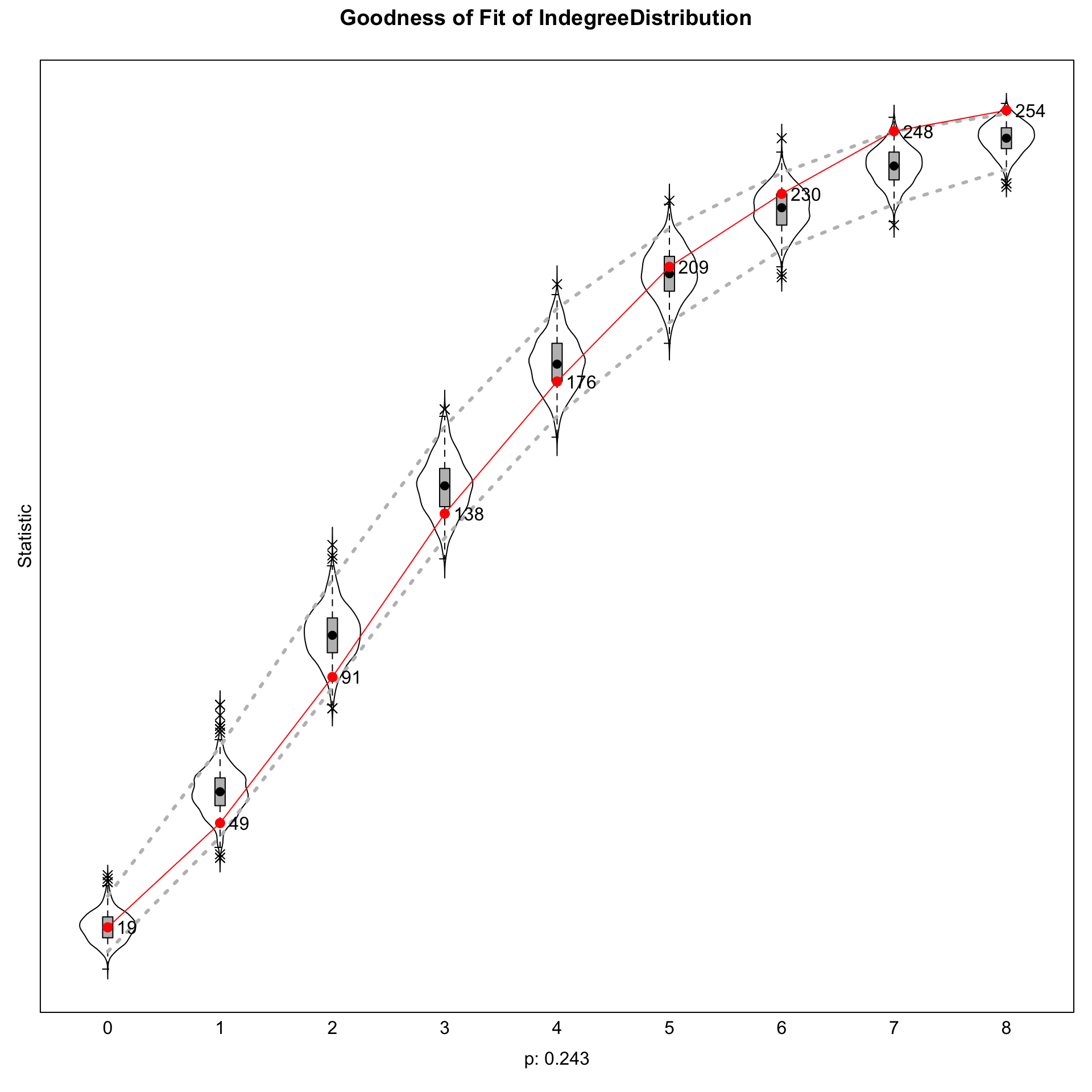
Interpret the figure by comparing the observed indegree distribution (solid line) with the distribution obtained from the simulated networks (boxplots).
Goodness of fit: Smoking behavior
Next, we assess whether the model reproduces the observed distribution of smoking behavior.
gof_behavior <- sienaGOF(
  result3,
  BehaviorDistribution,
  varName = "smoking"
)

plot(gof_behavior)
Note: some statistics are not plotted because their variance is 0.
This holds for the statistic: 3.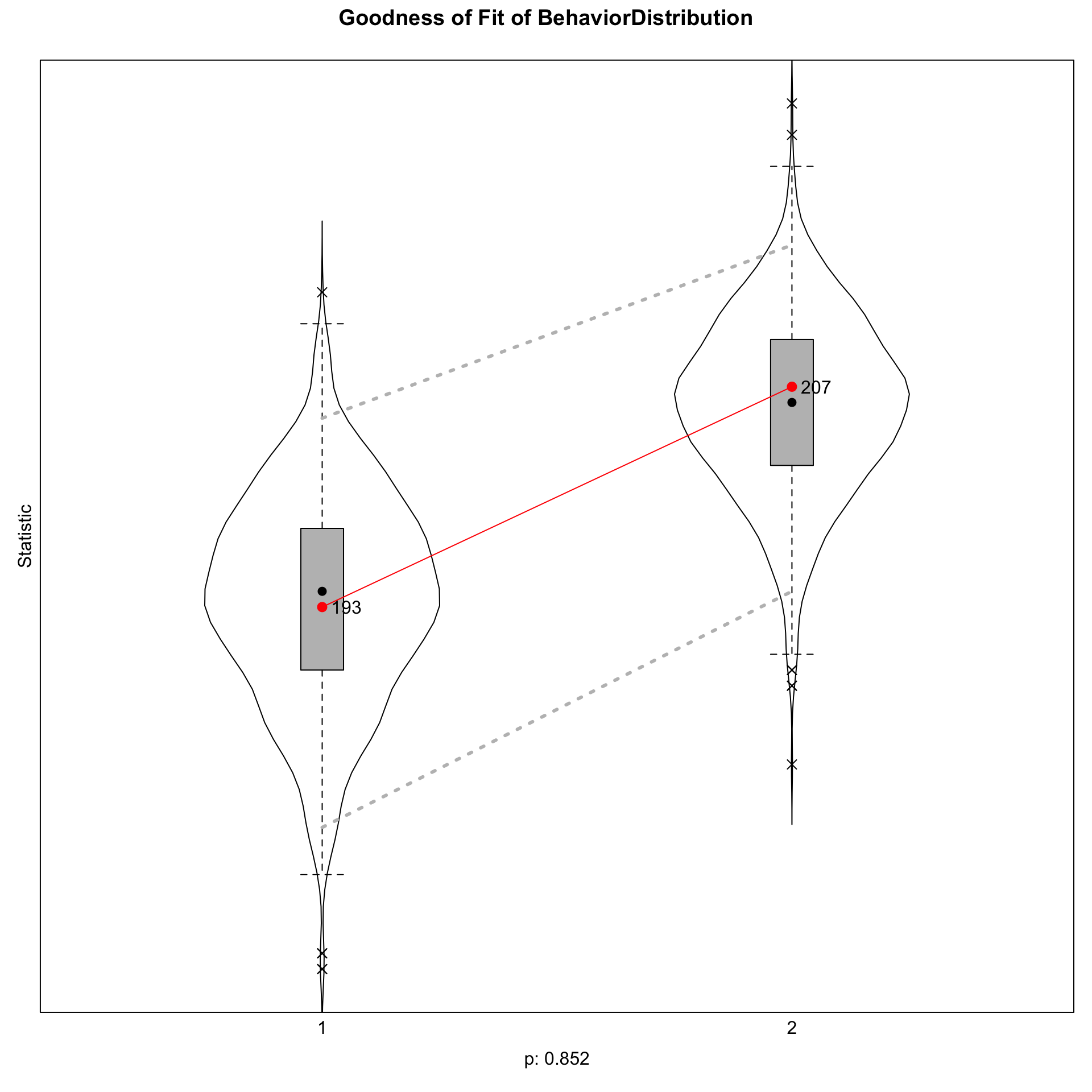
Again, compare the observed behavior distribution with the simulated distributions.
Why assess goodness of fit for smoking behaviour?
Although smoking behaviour is modelled directly in Model 3, it is still useful to assess its goodness of fit. The estimated parameters are chosen to explain how smoking changes over time, not to perfectly reproduce every feature of the observed data.
A behavioural goodness-of-fit check asks whether simulations from the fitted model generate a distribution of smoking behaviour similar to the one observed in the data. If the simulated and observed distributions are similar, this provides evidence that the model adequately captures the overall behavioural dynamics. If they differ substantially, the model may be missing important behavioural processes, even if individual parameter estimates appear reasonable.
The parameters in a SAOM define an actor-oriented objective function governing the micro-steps of network and behavioural change. The estimation procedure is not matching the final distribution of smoking behaviour in the same way an ERGM matches sufficient statistics. In other words, the ERGM is matching network statistics directly, whereas the SAOM is estimating a dynamic process whose consequences can still be checked using GOF diagnostics.
Discussion Questions
After estimating Model 3 (Co-evolution of Friendship and Smoking), answer the following questions.
Friendship dynamics: Is there evidence that friendship ties are shaped by reciprocity and transitive triplets? Interpret the estimated coefficients for these structural effects.
Network structure: What does the negative outdegree (density) parameter imply about the overall tendency to form friendships in the network?
Behavior dynamics: What do the linear shape and quadratic shape parameters indicate about changes in smoking behavior over time? Do they suggest that students tend to move toward lower, higher, or moderate levels of smoking?
Social influence: Does the average alter (
avAlt) effect provide evidence that students’ smoking behavior is influenced by the smoking behavior of their friends? Interpret both the sign and magnitude of this parameter.Statistical significance: Which estimated parameters appear to be statistically significant (using the estimates and standard errors)? What do these significant effects tell us about friendship evolution and smoking behavior?
Model convergence: Assess the convergence of the model.
What is the overall maximum convergence ratio?
Is it below the recommended threshold (preferably < 0.10, acceptable < 0.25)?
Based on the convergence diagnostics, would you consider the parameter estimates reliable? Explain your reasoning.
If convergence is poor, what changes to the model or estimation procedure might improve it?
Goodness of fit (Network): Does the fitted model adequately reproduce the indegree distribution? Use the goodness-of-fit plot to justify your answer.
Goodness of fit (Behavior): Does the fitted model adequately reproduce the distribution of smoking behavior? What aspects of the observed distribution are well captured, and where does the model perform poorly?
Overall assessment: Considering the parameter estimates, convergence diagnostics, and goodness-of-fit results, how well does the co-evolution SAOM explain the joint evolution of friendship ties and smoking behavior? What limitations of the model remain?
Social influence
Finally we estimate peer influence.
This tests whether students tend to become more similar to the average smoking behavior of their friends.